Multiobjective evolutionary optimization

This example shows how to run the optimization algorithms contained in the evoalgos package. It optimises four typical SWIM parameters to the (reversed) NSE and absolute bias at the Blankenstein station.

Prerequisites

The objective functions used here (NSE and pbias) rely on observed discharge, i.e. make sure the stations are properly setup in the swimpy/settings.py file.

import swimpy

objectives = ['subbasin_label_daily_selected_stations_discharge.rNSE.BLANKENSTEIN',
              'subbasin_label_daily_selected_stations_discharge.pbias_abs.BLANKENSTEIN']

# low, high ranges
parameters = {'smrate': (0.2, 0.7),
              'sccor': (0.1, 10),
              'ecal': (0.7, 1.3),
              'roc2': (0.5, 10)}

# load the project instance
p = swimpy.Project()

# this works for local runs
p.settings(cluster_run_parallel_parallelism='mp')

# silence swim
p.config_parameters(log_stdout_level='error',
                    log_stderr_level='error')

# adjust runtime and make sure subcatch is switched off
p.config_parameters(nbyr=2)

# runs swim 10 x 10 times using all available CPU cores
run = p.SMSEMOA(parameters, objectives, population_size=10, max_generations=10)

Visualising the results

from matplotlib import pyplot as plt

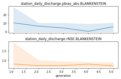
# development of objective functions with generations
_ = run.optimization_populations.plot_generation_objectives()

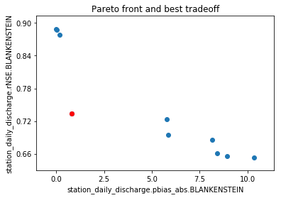
# the Pareto front with the 'best tradeoff' marked
run.optimization_populations.plot_objective_scatter(best=True)
title = plt.title('Pareto front and best tradeoff')

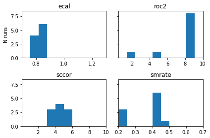
# parameter distribution
_ = run.optimization_populations.plot_parameter_distribution()

Download as Notebook